One-Way Analysis of Variance (ANOVA) for Within-Subject or Repeated Measures Designs
One-Way Analysis of Variance (ANOVA) for Within-Subject or Repeated Measures Designs


Purpose:
To determine whether there is a significant difference between multiple treatments or conditions within the same group of participants over time or across different variables.
Assumptions:
Normally distributed data
Homogeneity of variances
Independence of observations
Sphericity (for repeated measures)
Example:
Descriptive Statistics
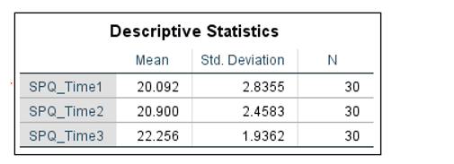
The descriptive statistics that
SPSS outputs are easy enough to understand. The comparison between means (see
above) gives us an idea of the direction of any possible effect. In our
example, it seems as if fear of spiders increases over time, with the greatest
increase (20.90 to 22.26 on the SPQ scale) occurring between year 1 (SPQ_Time2)
and year 2 (SPQ_Time3). Of course, we won’t know whether these differences in
the means reach significance until we look at the result of the ANOVA test.
Assumption of
Sphericity
A requirement that must be met before you can
trust the p-value generated by the standard
repeated-measures ANOVA is the homogeneity-of-variance-of-differences (or
sphericity) assumption. For our purposes, it doesn’t matter too much what this
means, we just need to know how to figure out whether the requirement has been
satisfied.
SPSS tests this
assumption by running Mauchly’s test of sphericity.
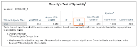
What we’re looking for here is a p-value that’s greater than
.05. Our p-value is .494, which means we meet the assumption of
sphericity.
Tests of Within-Subjects Effects
This is where we read off the
result of the repeated-measures ANOVA test.
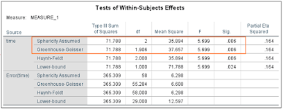
As we have just discussed, our
data meets the assumption of sphericity, which means we can read our result
straight from the top row (Sphericity Assumed). The value of F is 5.699,
which reaches significance with a p-value of .006
(which is less than the .05 alpha level). This means there is a statistically
significant difference between the means of the different levels of the
within-subjects variable (time).
If our data had not met the
assumption of sphericity, we would need to use one of the alternative
univariate tests. You’ll notice that these produce the same value for F, but that there
is some variation in the reported degrees of freedom. In our case, there is not
enough difference to alter the p-value –
Greenhouse-Geisser and Huynh-Feldt, both produce significant results (p = .006).
Pairwise
Comparisons
Although
we know that the differences between the means of our three within-subjects
levels are large enough to reach significance, we don’t yet know between which
of the various pairs of means the difference is significant. This is where
pairwise comparisons come into play.
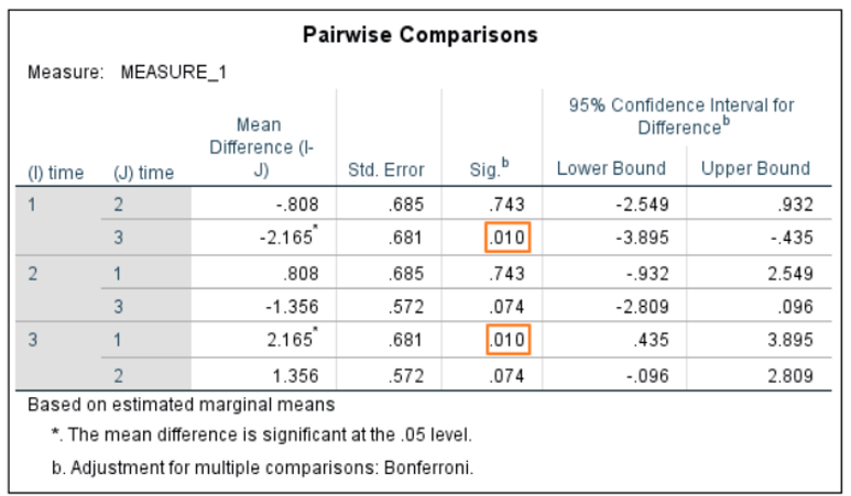
This table
features three unique comparisons
between the means for SPQ_Time1, SPQ_Time2 and SPQ_Time3. Only one of the
differences reaches significance, and that’s the difference between the means
for SPQ_Time1 and SPQ_Time 3 (see above). It is worth noting that SPSS is using
an adjusted p-value here
in order to control for multiple comparisons, and that the program lets you
know if a mean difference has reached significance by attaching an asterisk to
the value in column 3.
Report the Result
When reporting the result it’s
normal to reference both the ANOVA test and any post hoc analysis that has been
done.
Thus, given our example, you
could write something like:
A repeated-measures ANOVA determined that mean SPQ scores
differed significantly across three time points (F(2, 58) = 5.699, p = .006). A
post hoc pairwise comparison using the Bonferroni correction showed an
increased SPQ score between the initial assessment and follow-up assessment one
year later (20.1 vs 20.9, respectively), but this was not statistically
significant (p = .743).
However, the increase in SPQ score did reach significance when comparing the
initial assessment to a second follow-up assessment taken two years after the
original assessment (20.1 vs 22.26, p = .010). Therefore, we can conclude that
the results for the ANOVA indicate a significant time effect for untreated fear
of spiders as measured on the SPQ scale.
Procedure:
1. Formulate the hypothesis:
Null hypothesis (H0): There is no significant difference between the treatments/conditions.
Alternative hypothesis (Ha): There is a significant difference between the treatments/conditions.
2. Collect data:
Gather data on the response variable for each participant in each treatment/condition.
3. Calculate the following statistics:
Within-subject effect (SSW): Sum of squares of deviations from the grand mean
Between-subject effect (SSB): Sum of squares of deviations between group means
Error effect (SSE): Sum of squares of residuals
Mean square within (MSW): SSW divided by the degrees of freedom for within-subject effect (n-1)
Mean square between (MSB): SSB divided by the degrees of freedom for between-subject effect (k-1)
F-statistic: MSB divided by MSW
4. Test the hypothesis:
Calculate the F-statistic and compare it to the critical value for the F-distribution with degrees of freedom (k-1) and (n-1)(k-1).
If the F-statistic exceeds the critical value, reject the null hypothesis.
5. Post-hoc tests:
If the ANOVA is significant, conduct post-hoc tests to determine which pairs of treatments/conditions are significantly different from each other.
Commonly used tests include Tukey's HSD, Bonferroni, and Scheffé.
Advantages:
Powerful test for detecting differences between multiple treatments/conditions.
Controls for individual differences between participants.
Disadvantages:
Requires balanced data with an equal number of participants in each treatment/condition.
Assumes sphericity, which can be violated in certain designs.
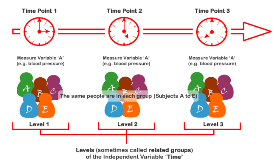
ANOVA is a statistical technique used to compare the means of multiple groups when there is a single independent variable with two or more levels. In a within-subject or repeated measures design, participants are measured on multiple occasions under different conditions.
Applications in Health:
Drug trials: Comparing the effectiveness of different drug regimens.
Treatment efficacy: Assessing the difference in clinical outcomes before and after an intervention.
Longitudinal studies: Monitoring the change in health parameters over time.
Example:
Consider a study investigating the effects of a new exercise program on blood pressure. Participants' blood pressure is measured at baseline (Time 1) and after 6 weeks of the program (Time 2).
ANOVA Procedure:
1. Calculate the within-subject variance: This represents the variability in participants' blood pressure over time.
2. Calculate the between-subject variance: This represents the variability in blood pressure between participants.
3. Compare the variances: Using an F-test, determine if the between-subject variance is significantly greater than the within-subject variance.
4. If there is a significant difference: Conduct post-hoc tests (e.g., paired t-tests) to determine which specific time points differ significantly.
Interpretation:
A significant ANOVA result indicates that there is at least one significant difference in blood pressure between Time 1 and Time 2.
Post-hoc tests can then be used to determine which specific time points show significant differences.
Advantages:
Allows for comparisons of multiple conditions within the same participants.
Reduces the impact of between-subject variability.
Can detect changes over time or in response to interventions.
Note:
Assumptions must be met for ANOVA to be valid, including normality of the residuals and homogeneity of variances.
Alternative statistical techniques, such as linear mixed models, may be more appropriate for handling unbalanced or missing data.
Example:
A researcher wants to investigate the effect of three different study techniques on the test scores of students. Each student is tested on three different occasions using the different study techniques. An ANOVA for within-subject design is conducted to test whether there is a significant difference in test scores between the three techniques.
......................................................................................................
👉 For the data analysis, please go to my Youtube(Ads) channel to Watch Video (Video Link) in
Youtube Channel (Channel Link) and Download(Ads) video.
💗 Thanks to Subscribe(channel) and Click(channel) on bell 🔔 to get more videos!💗!!
- Tell: (+855) - 96 810 0024
- Telegram: https://t.me/sokchea_yann
- Facebook Page: https://www.facebook.com/CambodiaBiostatistics/
- TikTok: https://www.tiktok.com/@sokcheayann999
.png)
- STATA for dataset restructuring, descriptive and analytical data analysis
- SPSS for dataset restructuring, data entry, data check, descriptive, and analytical data analysis
- Epi-Info for building questionnaires, data check, data entry, descriptive, and analytical data analysis
- Epidata-Analysis for dataset restructuring, descriptive and analytical data analysis
- Epi-Collect for building questionnaires, remote data entry, mapping, and data visualization
- Epidata-Entry for building questionnaires, data check, data entry, and data validation
ABA Account-holder name: Sokchea YAN
ABA Account number: 002 996 999
ABA QR Code:

or tap on link below to send payment:
https://pay.ababank.com/iT3dMbNKCJhp7Hgz6
✌ Have a nice day!!! 💞


Comments
Post a Comment